Generative Adversarial Networks Part 2 - Implementation with Keras 2.0
⌛ This article is quite old! This article dates back from when I was studying for my Master of Science in Machine Learning at Georgia Tech. Since then, I recentered my career away from the subject. While the subject here is interesting, I am clearly not an authoritative source on the subject and you should keep that in mind when looking at this article…
In this part, we’ll consider a very simple problem (but you can take and adapt this infrastructure to a more complex problem such as images just by changing the sample data function and the models). In our real sampled data, we’ll generate random sinusoid curves and we’ll try to make our GAN generate correct sinusoidal curves.
All of the code required to run the GAN is in this tutorial. All of the required imports are located at the end.
Getting the “real” data
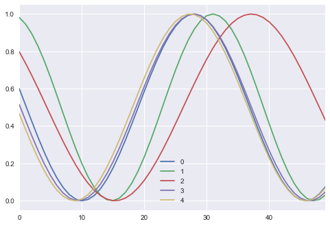
We just need to randomly generate curves, this is pretty simple to do. You can readapt this function to sample from a dataset if you want to take images for instance.
Here is the data sampling function:
def sample_data(n_samples=10000, x_vals=np.arange(0, 5, .1), max_offset=100, mul_range=[1, 2]):
    vectors = []
    for i in range(n_samples):
        offset = np.random.random() * max_offset
        mul = mul_range[0] + np.random.random() * (mul_range[1] - mul_range[0])
        vectors.append(
            np.sin(offset + x_vals * mul) / 2 + .5
        )
    return np.array(vectors)

ax = pd.DataFrame(np.transpose(sample_data(5))).plot()
Create the models
As we saw in the first part, we need to create a model that we will train to generate images from some noise and a model supposed to detect real data from generated data.
Generative model
We create our generative model using simple dense layers activated by tanh. This model will take noise and try to generate sinusoidals from it. This model will not be trained directly but trained via the GAN.
def get_generative(G_in, dense_dim=200, out_dim=50, lr=1e-3):
    x = Dense(dense_dim)(G_in)
    x = Activation('tanh')(x)
    G_out = Dense(out_dim, activation='tanh')(x)
    G = Model(G_in, G_out)
    opt = SGD(lr=lr)
    G.compile(loss='binary_crossentropy', optimizer=opt)
    return G, G_out

G_in = Input(shape=[10])
G, G_out = get_generative(G_in)
G.summary()
_________________________________________________________________
Layer (type)                 Output Shape              Param #
=================================================================
input_1 (InputLayer)         (None, 10)                0
_________________________________________________________________
dense_1 (Dense)              (None, 200)               2200
_________________________________________________________________
activation_1 (Activation)    (None, 200)               0
_________________________________________________________________
dense_2 (Dense)              (None, 50)                10050
=================================================================
Total params: 12,250.0
Trainable params: 12,250.0
Non-trainable params: 0.0
_________________________________________________________________
Discriminative model
Similarly, we create our discriminative model that will define if the curve is real or outputted by the generative model. This one, though will be trained directly.
def get_discriminative(D_in, lr=1e-3, drate=.25, n_channels=50, conv_sz=5, leak=.2):
    x = Reshape((-1, 1))(D_in)
    x = Conv1D(n_channels, conv_sz, activation='relu')(x)
    x = Dropout(drate)(x)
    x = Flatten()(x)
    x = Dense(n_channels)(x)
    D_out = Dense(2, activation='sigmoid')(x)
    D = Model(D_in, D_out)
    dopt = Adam(lr=lr)
    D.compile(loss='binary_crossentropy', optimizer=dopt)
    return D, D_out

D_in = Input(shape=[50])
D, D_out = get_discriminative(D_in)
D.summary()
_________________________________________________________________
Layer (type)                 Output Shape              Param #
=================================================================
input_2 (InputLayer)         (None, 50)                0
_________________________________________________________________
reshape_1 (Reshape)          (None, 50, 1)             0
_________________________________________________________________
conv1d_1 (Conv1D)            (None, 46, 50)            300
_________________________________________________________________
dropout_1 (Dropout)          (None, 46, 50)            0
_________________________________________________________________
flatten_1 (Flatten)          (None, 2300)              0
_________________________________________________________________
dense_3 (Dense)              (None, 50)                115050
_________________________________________________________________
dense_4 (Dense)              (None, 2)                 102
=================================================================
Total params: 115,452.0
Trainable params: 115,452.0
Non-trainable params: 0.0
_________________________________________________________________
Chained model: GAN
Finally, we chain the two models into a GAN that will serve to train the generator while we freeze the discriminator.
In order to freeze the weights of a given model, we create this freezing function that we will apply on the discriminative model each time we train the GAN, in order to train the generative model.
def set_trainability(model, trainable=False):
    model.trainable = trainable
    for layer in model.layers:
        layer.trainable = trainable

def make_gan(GAN_in, G, D):
    set_trainability(D, False)
    x = G(GAN_in)
    GAN_out = D(x)
    GAN = Model(GAN_in, GAN_out)
    GAN.compile(loss='binary_crossentropy', optimizer=G.optimizer)
    return GAN, GAN_out

GAN_in = Input([10])
GAN, GAN_out = make_gan(GAN_in, G, D)
GAN.summary()
_________________________________________________________________
Layer (type)                 Output Shape              Param #
=================================================================
input_3 (InputLayer)         (None, 10)                0
_________________________________________________________________
model_1 (Model)              (None, 50)                12250
_________________________________________________________________
model_2 (Model)              (None, 2)                 115452
=================================================================
Total params: 127,702.0
Trainable params: 12,250.0
Non-trainable params: 115,452.0
_________________________________________________________________
Training
Now we did setup our models, we can train the models by alterning training the discriminator and the chained models.
Pre-training
Let’s now generate some fake and real data and pre-train the discriminator before starting the gan. This also let us check if our compiled models correclty runs on our real and noisy input.
def sample_data_and_gen(G, noise_dim=10, n_samples=10000):
    XT = sample_data(n_samples=n_samples)
    XN_noise = np.random.uniform(0, 1, size=[n_samples, noise_dim])
    XN = G.predict(XN_noise)
    X = np.concatenate((XT, XN))
    y = np.zeros((2*n_samples, 2))
    y[:n_samples, 1] = 1
    y[n_samples:, 0] = 1
    return X, y

def pretrain(G, D, noise_dim=10, n_samples=10000, batch_size=32):
    X, y = sample_data_and_gen(G, n_samples=n_samples, noise_dim=noise_dim)
    set_trainability(D, True)
    D.fit(X, y, epochs=1, batch_size=batch_size)

pretrain(G, D)
Epoch 1/1
20000/20000 [==============================] - 3s - loss: 0.0078
Alternating training steps
We can now train our GAN by alternating the training of the Discriminator and the training of the chained GAN model with Discriminator’s weights freezed.
def sample_noise(G, noise_dim=10, n_samples=10000):
    X = np.random.uniform(0, 1, size=[n_samples, noise_dim])
    y = np.zeros((n_samples, 2))
    y[:, 1] = 1
    return X, y

def train(GAN, G, D, epochs=500, n_samples=10000, noise_dim=10, batch_size=32, verbose=False, v_freq=50):
    d_loss = []
    g_loss = []
    e_range = range(epochs)
    if verbose:
        e_range = tqdm(e_range)
    for epoch in e_range:
        X, y = sample_data_and_gen(G, n_samples=n_samples, noise_dim=noise_dim)
        set_trainability(D, True)
        d_loss.append(D.train_on_batch(X, y))

        X, y = sample_noise(G, n_samples=n_samples, noise_dim=noise_dim)
        set_trainability(D, False)
        g_loss.append(GAN.train_on_batch(X, y))
        if verbose and (epoch + 1) % v_freq == 0:
            print("Epoch #{}: Generative Loss: {}, Discriminative Loss: {}".format(epoch + 1, g_loss[-1], d_loss[-1]))
    return d_loss, g_loss

d_loss, g_loss = train(GAN, G, D, verbose=True)
Epoch #50: Generative Loss: 4.795285224914551, Discriminative Loss: 0.49175772070884705
Epoch #100: Generative Loss: 3.5881073474884033, Discriminative Loss: 0.05777553841471672
Epoch #150: Generative Loss: 3.3537204265594482, Discriminative Loss: 0.23116469383239746
Epoch #200: Generative Loss: 3.221881151199341, Discriminative Loss: 0.11503896117210388
Epoch #250: Generative Loss: 3.9224398136138916, Discriminative Loss: 0.06002074107527733
Epoch #300: Generative Loss: 3.3472070693969727, Discriminative Loss: 0.08401770144701004
Epoch #350: Generative Loss: 3.591559648513794, Discriminative Loss: 0.04007931426167488
Epoch #400: Generative Loss: 3.796259880065918, Discriminative Loss: 0.03941405192017555
Epoch #450: Generative Loss: 4.634820938110352, Discriminative Loss: 0.022133274003863335
Epoch #500: Generative Loss: 3.2044131755828857, Discriminative Loss: 0.05611502751708031
ax = pd.DataFrame(
    {
        'Generative Loss': g_loss,
        'Discriminative Loss': d_loss,
    }
).plot(title='Training loss', logy=True)
ax.set_xlabel("Epochs")
ax.set_ylabel("Loss")
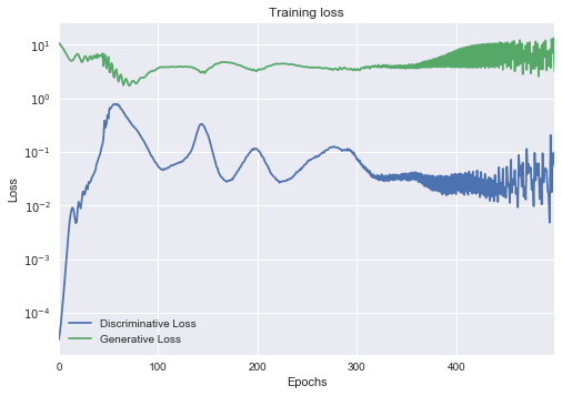
What is interesting here is that both sides are playing with each other, each learning how to get better than the other. We see that during some phases, either the generator or the discriminator is lowering its loss relative to a loss gain on the other side.
Watching the loss of the models does not seem to have a huge importance to quantify the progress in quality of the models. We actually don’t really want to have models converging to zero too fast, otherwise, that means that they managed to trick each other. However the amount of times each model got better relatively to the other may be an interesting metric. to watch.
Results
We can now vizualize some generated sinusoidal curves from our generator:
N_VIEWED_SAMPLES = 2
data_and_gen, _ = sample_data_and_gen(G, n_samples=N_VIEWED_SAMPLES)
pd.DataFrame(np.transpose(data_and_gen[N_VIEWED_SAMPLES:])).plot()
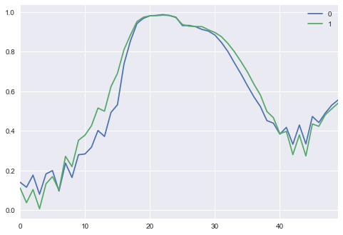
This is not perfect, however, we see that if we smooth a bit the curve using a rolling mean, we approach a more precise sinusoidal shape.
N_VIEWED_SAMPLES = 2
data_and_gen, _ = sample_data_and_gen(G, n_samples=N_VIEWED_SAMPLES)
pd.DataFrame(np.transpose(data_and_gen[N_VIEWED_SAMPLES:])).rolling(5).mean()[5:].plot()
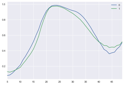
Obviously with more training and more tuning, we could get better results. A greater amount of epochs usually prooves to be efficient on a GAN, but it would be long to run in a simple tutorial like this one.
Finally, we see that the generator does not takes many risks and will more or less output the same curve for different noise input. This is to be expected, our very simple model will prefer refining something it already knows to do instead of trying something new. This is a risk with GANs that can be mitigated with more varied data but will require more training overall (and a good GPU if you want this training to finish one day…).
Conclusion
Creating GANs on keras is not a really hard task technically since all you have to do is create those 3 models and define how to do a training step with them but depending on the task you may want to achieve, more or less tuning and computations will be required.
GANs are overall very powerful but may be very hard to tune correctly especially since measuring how well they do is hard. The loss is not necessarily a good indicator and for now, the most reliable way to check if their output makes sense is to put the output in front of an actual person.
References
Imports
%matplotlib inline
import os
import random
import numpy as np
import pandas as pd
import matplotlib.pyplot as plt
import seaborn as sns
from tqdm import tqdm_notebook as tqdm
from keras.models import Model
from keras.layers import Input, Reshape
from keras.layers.core import Dense, Activation, Dropout, Flatten
from keras.layers.normalization import BatchNormalization
from keras.layers.convolutional import UpSampling1D, Conv1D
from keras.layers.advanced_activations import LeakyReLU
from keras.optimizers import Adam, SGD
from keras.callbacks import TensorBoard